How To Draw Butterfly Chart In Excel

Open Excel and select New Workbook. Create a data set in the excel sheet with the product name and the values.

Best Excel Tutorial Butterfly Chart

In Chart Area select Vertical Category Axis press Delete.

How to draw butterfly chart in excel. See the screenshot below. In Select Data Source window select Gap series click Move Up once. In the Select Data window click on Legend Entries and enter Category in the name input bar.

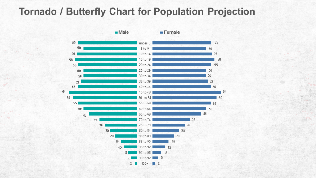
Click on the arrows to sort the series Padding South South Gap North and Padding North 1 and press ok 2. Select All Charts while inserting the chart. 04062019 The excel tornado chart is also known as the Butterfly chart.

First of all go to Insert Tab Charts Doughnut Chart with this youll get a blank chart. Click on Add chart element 1 Legends 2 and Top 3. On the Insert tab in the Charts group click the Histogram symbol.

17062014 Your chart should look like the one below at this point. Click on the Insert tab present on the uppermost ribbon in the Microsoft Excel sheet and select the Recommended Charts option out of it. Click the button on the right side of the chart and click the check box next to Data Labels.

Right click on one of the series 1 and Select Data 2. Select the X Y Scatter and you can select the pre-defined graphs to start quickly. Add labels to remaining data series.

You can see the built-in styles at the top of the dialog box. Click on the third style Scatter with Smooth Lines. This example shows you how to make the chart look like a butterfly chart.

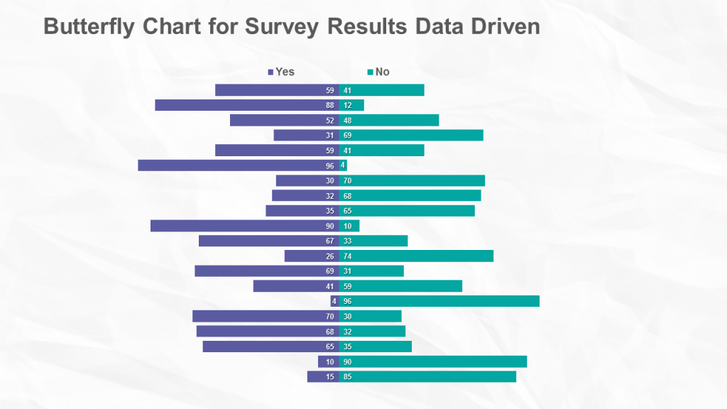
This example explains an alternate approach to arrive at a combination chart in Excel. 29092020 To create a SPEEDOMETER in Excel you can use the below steps. For Yes orange series select position as Inside End and for No yellow series select position as Inside Base.

Enter the data you want to use to create a graph or chart. Go to the Insert tab and click on Recommended Charts. From here select the axis label and open formatting options and in the formatting options go.

Enter a chart title. In this section well show you how to chart data in Excel 2016. Step 1- First select the data table prepared then go to the insert tab in the ribbon click on Combo and then select clustered column line.

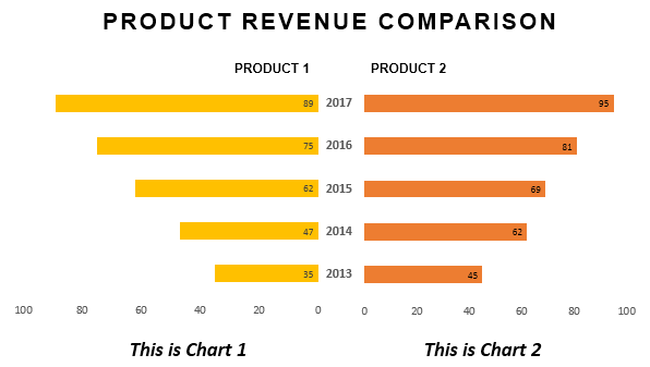
In order to create a graph associated with your data select all the data from A1 to F6. Go to Insert Tab Charts Bar Chart and with this youll get a bar chart like below where you have two sides one is side is for positive values and another is for negative. Right click on padding North 1 and click on no fill 2.

Once you click on the Recommended Charts option it will. 21062014 In Chart Area Right click and choose Select Data. Enter Data into a Worksheet.

Just add another column in the data set with the column name as GAP after the variables column. Once the clustered chart is selected the combo chart would be ready for display and illustration. 22012018 To generate a chart or graph in Excel you must first provide Excel with data to pull from.

Now right-click on the chart and then click on Select Data. A Pareto chart combines a column chart and a line graph. Also select Gap series which is in the middle invisible and add labels.

In Format Data Series window click Fill tab click No Fill then click Close. In Chart Area select Series GAP press CTRL1.

How To Create A Butterfly Chart Tornado Chart In Powerpoint The Slideteam Blog